Fitting curves
The routine used for fitting curves is part of the scipy.optimize module
and is called scipy.optimize.curve_fit(). So first said module has to be
imported.
>>> import scipy.optimize
The function that you want to fit to your data has to be defined with the x
values as first argument and all parameters as subsequent arguments.
>>> def parabola(x, a, b, c):
...     return a*x**2 + b*x + c
...
For test purposes the data is generated using said function with known parameters.
>>> params = [-0.1, 0.5, 1.2]
>>> x = np.linspace(-5, 5, 31)
>>> y = parabola(x, params[0], params[1], params[2])
>>> plt.plot(x, y, label='analytical')
[<matplotlib.lines.Line2D object at ...>]
>>> plt.legend(loc='lower right')
<matplotlib.legend.Legend object at ...>
>>> plt.show()

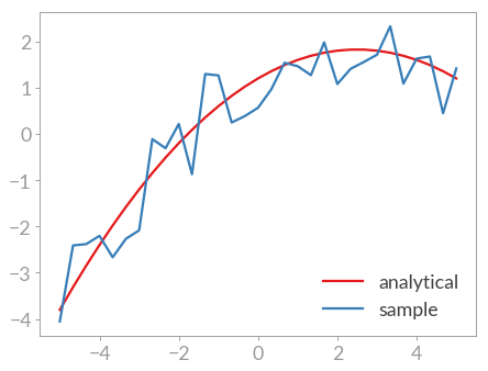
Then some small deviations are introduced as fitting a function to data generated by itself is kind of boring.
>>> r = np.random.RandomState(42)
>>> y_with_errors = y + r.uniform(-1, 1, y.size)
>>> plt.plot(x, y_with_errors, label='sample')
[<matplotlib.lines.Line2D object at ...>]
>>> plt.legend(loc='lower right')
<matplotlib.legend.Legend object at ...>
>>> plt.show()
Now the fitting routine can be called.
>>> fit_params, pcov = scipy.optimize.curve_fit(parabola, x, y_with_errors)
It returns two results, the parameters that resulted from the fit as well as the covariance matrix which may be used to compute some form of quality scale for the fit. The actual data for the fit may be compared to the real parameters:
>>> for param, fit_param in zip(params, fit_params):
...     print(param, fit_param)
...
-0.1 -0.0906682795944
0.5 0.472361903203
1.2 1.00514576223
>>> y_fit = parabola(x, *fit_params)
>>> plt.plot(x, y_fit, label='fit')
[<matplotlib.lines.Line2D object at ...>]
>>> plt.legend(loc='lower right')
<matplotlib.legend.Legend object at ...>
>>> plt.show()
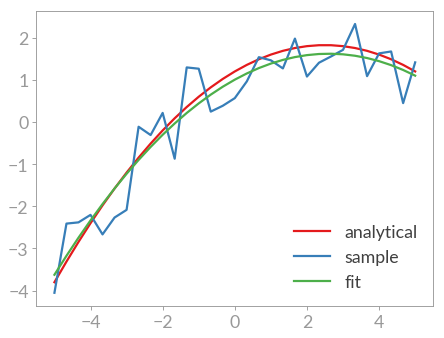
As you can see the fit is rather off for the third parameter c. A look at
the covariance matrix also shows this:
>>> print(pcov)
[[  1.64209005e-04   1.75357845e-12  -1.45963560e-03]
 [  1.75357845e-12   1.16405938e-03  -1.73642112e-11]
 [ -1.45963560e-03  -1.73642112e-11   2.33217333e-02]]
But to get a more meaningful scale for the quality of the fit the documentation recommends the following:
>>> print(np.sqrt(np.diag(pcov)))
[ 0.01281441  0.03411831  0.15271455]
So the fit for a is quite well whereas the quality c is the worst of
all the parameters.
Note
This routine works by iteratively varying the parameters and checking
whether the fit got better or worse. To help the routine find the best fit
it is hence a good idea to give it a good starting point. this can be done
using the p0 argument of curve_fit(). In some
cases this is even necessary.